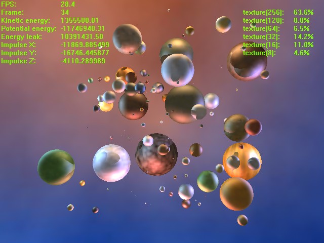
The CPU RightMark suite is meant for objective measurement of performance of modern and future processors in different computational tasks such as numerical modeling of physical processes and solving of 3D graphic problems. It focuses on testing the loaded FPU/SIMD units and the CPU/RAM tandem. As a result, we get pure CPU performance, an objective parameter obtained without the influence of other subsystems, like video and disc systems, except the memory one. It allows us to compare the true performance of different processors irrespective of a type of other system components. It's obtained by dealing only with the CPU and measuring the CPU time spent for execution of computational tasks. Thanks to high accuracy of measurements it takes less than one minute to obtain stable repeatable results.

The current CPU RightMark version consists of two tests - CPU Performance and CPU Stability.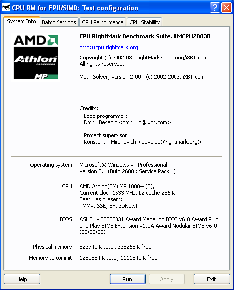 

CPU Performance

The first test deals with both types of tasks - numeric modeling of physical processes and 3D graphics. The calculation of a system of particles is displayed as a beautiful scene that consists of multiple spheres. Therefore, the CPU Performance test can be divided into two independent modules running one after the other.

1. Numeric modeling

The first module (Solver) realizes numeric modeling of physical processes. Initialization of this module sets a number of the particles to be computed, their initial coordinates in the environment, their speeds and accelerations (as a rule, the latter is equal to 0 at the initial moment of time), their mass and radii, parameters of the interaction potential (lin_factor and quad_factor) and the factor of energy loss due to friction (v_factor).

Potential of particles' interaction

The parameters depend on the model of interaction of particles selected in the test settings (see their description below).

Solver estimates interaction of the particles at every step to get new acceleration values for every particle and then solves the classical motion equation.

Equations of motion of particles 

As a result, we get new speeds and coordinates of the particles, energy and momentum of the whole system, which are displayed as the test goes on. The procedure of estimation of the interaction and calculation of the motion equations repeats several times, and the number of iterations and dt (time step) can vary.

The calculations in this module are carried out with double-precision variables. That is why Solver realizes three versions of the code optimization. The first uses x87 FPU, two others use SIMD extensions handling double-precision variables - SSE2 (available in Intel Pentium 4 and AMD Opteron/Athlon 64/FX) and SSE3 (in Intel Pentium 4 Prescott). The latter differs from SSE2 in a new operation of elementwise addition of components of the SSE2 register. Besides, every version of Solver intended for a certain instruction set realizes four versions of estimation of interaction of particles which differ in the number of manual code optimizations, and therefore, in performance. The CPU Performance test uses the highest-perfprmance version.

2. Scene rendering

The coordinates of the particles calculated by Solver go to the second module of CPU RightMark - Renderer. Initialization of this module is also very simple - it takes place when the test is run and the model type is selected. The constant parameters of spherical particles like their effective radius (which can differ from the actual radius), and the surface properties (diffuse and specular constants) are also selected at this moment. All other parameters - positions of particles, light sources and source colors - are selected anew for each frame, i.e. the can vary in time.

So, Renderer also does very important job - it calculates and renders a dynamic scene that consists of multiple spheres. Since the CPU RightMark focuses on performance of exactly the CPU, not a video system, the rendering method must be appropriate. I.e. it must use only the CPU, and but at same time it mustn't be very slow and it's desirable that its image quality didn't yield to the standard rendering methods of 3D accelerators. The best method is this respect is the back ray tracing. The rendering procedure can be divided into two parts - preliminary scene analysis (prerendering) and ray tracing (rendering).

At the prerendering stage the coordinates of particles (spheres) and light sources change relative the camera and direction of viewing. Then it clips off hidden spheres by checking if the sphere's center gets into the viewing pyramid (as a rule, in the realized models all spheres get into the viewing pyramid).

The next stage is distribution of the sphere indices among the screen (projection) space fields - small squares called tiles. It cuts down the expenses for searching the primary ray crossing in the following rendering procedure. When the area is divided like that, the program doesn't need to calculate where all spheres are crossed for each screen pixel, it deals only with the spheres that hit a given tile.

The last stage is the most complicated and CPU-intensive: calculation of lighting and shadowing of the spheres. An array of spheres is created for every light source according to its work range. After that the test checks each pair of spheres whether the first sphere can potentially shade the other, and vice versa. Then it creases a list of light sources for each sphere which can potentially light it, and a list of spheres which can shade a given light source (even partly) for each sphere/light source pair. Like partitioning of the screen area into tiles, this procedure cuts down the expenses for defining where the spheres are crossed by the secondary, or "shady", rays emitted from a given point of the visible sphere toward the light source.

Now comes the second Renderer procedure - back ray tracing. Since all necessary data are obtained at the prerendering stage, the ray tracing procedure is pretty simple. It goes from one pixel to another, and if the tile with a given pixel is empty (no sphere indices) this pixel can be considered processed and can be shaded with a respective element of the sky texture (or left empty if sky shading is disabled). If a tile contains sphere indices it defines where the ray emitted from the camera to a given screen pixel crosses all spheres that hit this tile and then defines the nearest one. Actually, they may not cross (for example, if a sphere hits only the lower right-hand tile corner, while the test calculates it for the upper left-hand one) - in this case it shades sky or doesn't shade anything at all. If a sphere is crossed by the ray the program initiates a long procedure to determine the color of a given pixel. 

If the scene texturing is set, the program calculates spherical texture coordinates and fetches a texture element (which becomes a diffuse scattering constant for this pixel, K_d), and it also calculates the ambient light component (K_a). Then it checks whether this sphere is lighted by any light sources. A ray (L) is emitted from a given pixel of the sphere for every light source, and the program checks whether it crosses potential shading spheres, until the first real value is found. This procedure is simpler than that with the primary rays because it must only ascertain whether it crosses spheres or not, without calculating the coordinates. If the ray crosses some sphere, this light source is shaded by another sphere and makes no contribution into lighting. Otherwise, this pixel of the sphere is lighted by this light source, and we need to calculate its luminance, for example, with the Fong model. The calculated illumination adds up with the overall illumination of this pixel.

Fong luminance model

Finally, the program records the obtained color into the frame buffer, and then repeats the ray tracing procedure for the next pixel.

For geometrical calculations Renderer uses single-precision real numbers (float), and processes color (texturing/lighting) with MMX extensions. Since single precision is sufficient for geometrical calculations the code can be optimized with SIMD extensions working with vectors of numbers of such type. The current CPU RightMark version features 5 Renderer versions. The first two use the standard x87 FPU and MMX extensions, as well as the addition to this set - MMX Extensions, which were for the first time available in Intel Pentium III (as a part of SSE) and early versions of AMD Athlon. The third version uses AMD Extended 3DNow! and Extended MMX extensions and, therefore, it can be used for comparing performance of the FPU and 3DNow! code on the first AMD Athlon models which do not support the SSE extensions. Finally, the last two Renderer modules use Intel SSE and SSE3 extensions and can serve an example of a fine manual code optimization. Thus, it realizes parallel processing of 4 scenes with calculation of shadowing correlations in prerendering and with searching where primary and secondary rays cross  spheres at the rendering stage. In the last case and additional speed gain is obtained at the expense of intensive utilization of horizontal addition instruction (HADDPS) which effectively calculates innerproduct of vectors which are many in number in the ray tracing procedure.

Finally, the ray tracing method allows for parallel calculations for pixels, even for the average one. But to get higher efficiency and avoid conflicts when different processors address the same memory area (in case of SMP systems) it's better to divide the screen into several parts and provide every processor (a physical or a logical one in HT systems) with its own part:

Multi-thread rendering

Such method tremendously increases the speed: the gain is almost proportional to the number of processors in SMP systems and makes up to 40% in the systems with Hyper-Threading support.

CPU Performance Test Settings

The CPU performance test has a lot of user settings which can vary in a very wide range. Below is the list of settings and descriptions for some of them.

Renderer Setup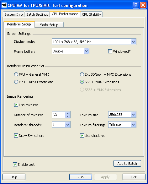

Screen Settings:

• Display Mode - screen resolution and refresh rate. The list of resolutions and refresh rates is based on the data provided by the video card driver to the DirectDraw subsystem.
• Frame Buffer. The double buffer consists of two buffers, one is displayed on the screen until the other is being filled up, then they interchange. The Triple buffer also contains a hidden one which can start receiving data without waiting until the current frame is totally displayed. Taking into account that scene rendering with the back ray tracing algorithm is slower than the refresh rate the Triple Buffering only causes extra consumption of the video memory. In the Offscreen Rendering mode a scene is rendered into a buffer located in the system memory, which is usually slower compared to utilization of the video memory. It happens because the CPU cache receives unnecessary data (results of pixel color calculation), and the video memory prevents it because it's based on the write-combining protocol that passes by the CPU cache levels system.
• Windowed - a scene is displayed in a window. The window size is fixed at 640x480 pixels. This mode is intended for debugging and is not available by default. It can be enabled in the system register key HKEY_CURRENT_USER\Software\RightMark\RMCPU\Tweak by setting Windowed value to: REG_DWORD = 1.

Renderer Instruction Set:

• FPU + General MMX (Intel Pentium MMX and higher).
• FPU + MMX Extensions (Intel Pentium III and higher, AMD Athlon and higher).
• Ext 3DNow! + MMX Extensions (AMD Athlon and higher).
• SSE + MMX Extensions (Intel Pentium III and higher, AMD Athlon XP/MP and higher).
• SSE3 + MMX Extensions (Intel Pentium 4 Prescott).

Image Rendering:

• Use Textures
• Number of textures:  1-32. Each sphere is given its own texture the number of which is equal to the number of the sphere modulo texture amount.
• Texture Size - maximum possible texture size (from 16x16 to 256x256). Since the MIP mapping is used the real texture size, especially in low resolutions, can be lower than the specified one. The test displays the texture distribution according to their sizes, percentagewise. Like the increase in the number of textures, the increase in their size results in a greater load on the cache/memory subsystem.

Distribution of textures according to their size

• Texture filtering. Bilinear filtering: a texture element is fetched using double linear interpolation of 4 neighbor pixels of the same texture's MIP level. Trilinear filtering is more advanced because the bilinear filtering is applied twice, for each of the neighbor MIP levels of the texture (thus, all eight pixels are involved into interpolation). The latter increases the load on the MMX unit and memory subsystem, which allows testing these components in harder conditions.
• Renderer threads. 1, 2, 4, 8 and 16 threads are possible; it allows measuring performance of a wide range of multiprocessor systems.
• Draw sky sphere. Since it usually takes a large part of the screen, and its rendering is as complicated as fetching texture elements for other spheres, if you disable this function, the rendering rate will noticeably grow up.
• Use shadows. When it's disabled, the program doesn't calculate sphere shades at the prerendering stage and crossing of shade rays at the rendering stage. It increases the rendering rate but the scene becomes less realistic.

Solver (Model Setup)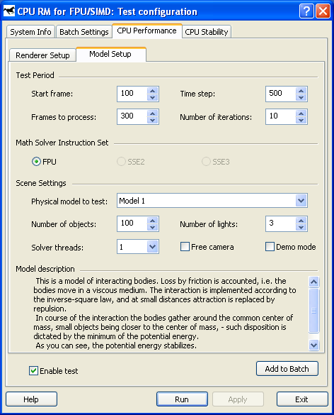

Test Period:

• Start frame - a number of the frame the performance measurement starts from.
• Frames to process - The number of frames for performance measurement. The total number of frames displayed equals the sum of these two values.
• Time step - a step of one iteration for motion equations, in microseconds.
• Number of iterations - for estimation of interaction/solving of motion equations.

Math Solver Instruction Set :

• FPU (supported by almost all processors).
• SSE2 (Intel Pentium 4, AMD Opteron/Athlon 64/FX).
• SSE3 (Intel Pentium 4 Prescott).

Scene Settings:

• Physical model to test - a type of the physical model of interacting bodies (1 - 7). Below are descriptions for each model.

  

Model 1
Loss by friction is accounted for, the bodies move in a viscous medium. They interact according to the law of inverse squares of distance, at a small distance attraction turns into repulsion. As the bodies interact they gather around the general center of mass, with the smaller bodies being closer to it. Such layout is explained by the minimum of potential energy. As the bodies interact the potential energy of the system stabilizes.

Model 2
Loss by friction is accounted for, the bodies move in a viscous medium. They interact according to the law of inverse distances, at a small distance attraction turns into repulsion. The configuration of objects becomes ball-like since such layout corresponds to the minimum of potential energy.

Model 3
No loss by friction. The bodies interact according to the law of inverse distances, at a small distance attraction turns into repulsion. The configuration of objects doesn't stabilize with time.

Model 4
No loss by friction. The bodies interact according to the law of inverse squares of distance, at a small distance attraction turns into repulsion. The configuration of objects doesn't stabilize with time.

Model 5
No loss by friction. The bodies interact according to the law of inverse squares of distance, at a small distance attraction turns into repulsion. The model is a star with a belt of asteroids. The configuration of objects doesn't stabilize with time. Because of such instability some asteroids fly away to infinity because of interaction at almost all initial conditions. Such behavior is typical of a system of multiple bodies that interact according to the law of inverse squares of radii, without friction (this is the physically accurate law of gravitational interaction). But the stability of configuration with one central body is pretty high and grows up as the central body becomes heavier.

Model 6
No loss by friction. The bodies interact according to the law of inverse distances, at a small distance attraction turns into repulsion. The model consists of three stars with a shared belt of asteroids. The configuration of objects doesn't stabilize with time but some of the objects do not fly away to infinity. Such behavior can be explained by the fact that the respective potential infinitely grows up at infinity. This model is an example of a system located in an infinitely deep potential well.

Model 7
Loss by friction is accounted for, the bodies move in a viscous medium. They interact according to the law of inverse distances, at a small distance attraction turns into repulsion. The configuration of objects becomes ball-like - such layout corresponds to the minimum of potential energy. Such behavior can be considered a demonstration of surface tension. And such model can also describe a drop of water.

• Number of objects. The increase in the number of objects results in quadratic increase of time of calculation of the system by Solver.
• Number of lights. It influences both the prerendering and rendering rates.
• Solver threads. The current version has only one possible value - 1 thread.
• Free camera - free camera control with keyboard and mouse. The camera is fixed by default, because it's useless to compare test results obtained in the free camera control mode.
• Demo mode - this mode allows using the test as a screensaver. The number of frames calculated is unlimited in this mode. The demonstration can be canceled with Escape key.

   

Besides, there are some extra demo mode settings located in the system register in HKEY_CURRENT_USER\Software\RightMark\RMCPU\Demo:

// statistics display (0 = off, 1 = on)
ShowInfo: REG_DWORD = 0

// periodic model randomization (0 = off, 1 = on)
RandomizeModel: DWORD = 1

// model randomization interval (number of frames)
RandomizeInterval: REG_DWORD = 200

// camera animation mode (0 = off, 1 = on)
CameraFly: REG_DWORD = 1

// camera animation direction (0 = counterclockwise, 1 = clockwise)
CameraCW: REG_DWORD = 1

// camera animation speed (1 - 10)
CameraSpeed: REG_DWORD = 3

The following system performance parameters are the final result of the first test:

Math Solving FPS - speed of computing the physics of a system of objects.
Prerendering FPS - speed of preliminary analysis.
Rendering FPS
Overall FPS - average speed (based on for three parameters).

CPU Stability Test

The second test of the CPU RightMark is intended for long testing of stability of the loaded CPU. The test uses the same task of numerical modeling executed by Solver. The measurement results are represented as a dependence of CPU performance on time. In particular, this test allows us to define the moment when the CPU clock falls down (throttling) when its temperature exceeds the limits, provided that the processors supports the Thermal Monitor temperature.

CPU Stability settings

These settings are very similar to the Solver settings in the first test, except some specific parameters.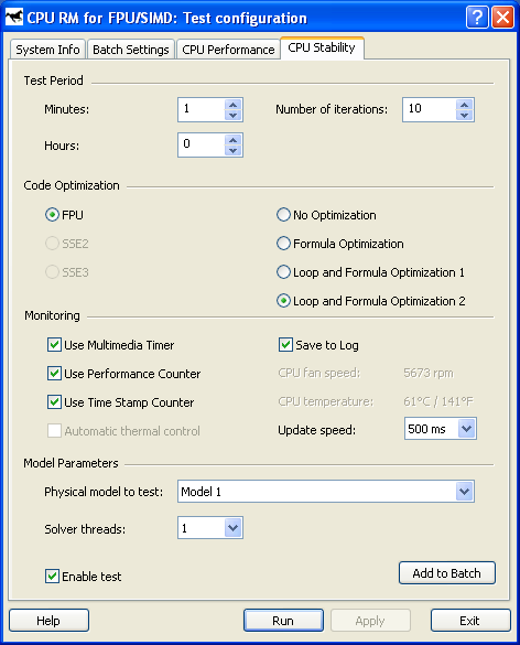

Test Period (Minutes, Hours), Solver parameters (Number of iterations).

Code Optimization - CPU extensions used (FPU, SSE2, SSE3), and the version of optimization of the interaction estimation:

• No Optimization.
• Formula Optimization.
• Loop and Formula Optimization 1 - formula optimization, unlooping, version 1.
• Loop and Formula Optimization 2 - formula optimization, unlooping, version 2.

Monitoring - performance measurement mode:

• Use Multimedia Timer - Standard Windows Multimedia Timer;
• Use Performance Counter - High-performance counter (HPC);
• Use Time Stamp Counter - CPU clock counter (TSC);
• Save to Log - saves measurement data into a file
• Update speed - diagram update speed (500, 1000 and 1500 ms);
• Automatic thermal control, CPU fan speed, CPU temperature - not realized yet.

Model Parameters - a model and the number of threads of Solver.

• Physical model to test - physical model (1 - 7). Each model is described above.
• Solver threads - the number of threads used by Solver. The current test version can set one or two threads. The main thread always makes calculations using FPU/SSE2/SSE3 CPU units while the second thread uses the ALU for integer calculations. This scheme is developed for more effective load on the Hyper-Threading systems.

Write a comment below. No registration needed!