Pic. 1 Brazil VFB and console settings
Laying aside purely artistic criteria, successful 3D scene render is determined by three main factors. These factors are good modelling, interesting materials, and lighting. And if modelling is out of the capacity of rendering programs, then materials and lighting are their direct responsibilities. These days there are several programs specializing in materials and lighting calculations. The most famous: mental ray, Vray, brazil r/s, finalrender, this list is constantly growing. Brazil takes its own worthy place among the modern rendering programs. Brazil possesses rather flexible and state-of-the-art illumination calculation capacities, though it's not the fastest renderer. Brazil has its own shader engine with universal interface. This engine is not as intricate as that in Renderman or in mental ray, which rely on programming necessary properties rather than on a library of ready shaders. However basic shader types in brazil have enough properties for a high-quality reproduction of material properties of the widest spectrum. In the production scale it makes brazil Choice #1 for small and medium studios, which have network rendering capacities and cannot or do not want to program their own shaders. However, brazil has a lot of sincere fans among individuals as well.
The object of this article is to review the main features and configuration peculiarities of illumination in brazil. And though we shall not review shaders in detail here, their influence on illumination will also be described where necessary.
Modern rendering algorithms allow to calculate many properties of real illumination. The entire calculation is usually divided into calculations of three main components. The first component is the calculation of direct illumination of objects from light sources, including lengthy objects in the line of sight. The second component, conditioned by reflection properties and material transparency, takes into account reflected or refracted illumination. At last, the third component – secondary illumination, conditioned by multiple diffuse reflections of direct light between object surfaces. Algorithms for calculating all the three components are well known and described in detail. That's why I will only provide their basics in order to preserve the continuity of the article.
All the three components are calculated separately and then are combined into one total result. The process starts with emitting rays from the camera (viewer) through a two-dimensional array of pixels, which form a future image, into the scene. The first cross point with the surface of a scene object is calculated for each ray. Then, the mentioned illumination components are calculated for all cross points. The total number of rays from the camera is specified by the antialiasing settings.
Direct illumination is calculated by emitting additional rays from each cross point in the direction of all light sources in the 3D scene. In this process the program determines whether the point is illuminated or in the shade and calculates distance to the light source and the angle between the direction to the light source and the normal of the cross point between the surface and the camera ray. If the scene contains not only spot lights, but also linear, area, or volume lights, a group of rays is emitted in their direction instead of a single ray, in order to determine to what degree the point is illuminated as the illumination total of different parts of the light source. This procedure allows to calculate "soft" or blurred borders between the shadow and light (penumbra). Area lights are the most widely used light sources in practice.
Reflected and refracted lights near the ideal refraction and reflection angles (mirror reflections) are calculated by means of raytracing. If the object surface possesses mirror reflection properties or transparency in the point it's crossed by the camera ray, another ray is calculated in the direction of ideal reflection and refraction angles or both, if the surface possesses both properties. New rays are traced to the next cross point with the scene object, where the procedure may be repeated, if the new cross point also possesses reflection/refraction properties. Rays from the starting point are traced until the specified raytracing depth is reached (the number of ray refractions specified in renderer settings). Or until the illumination contribution of the ray becomes less than a certain value. Illumination of the point from reflections and refractions is determined as a total illumination of all rays traced from this point. Modern modification of this algorithm allows to calculate diffuse reflections and refractions. This can be done because several rays are emitted from the starting point (instead of a single ray) in the range of angles close to the ideal reflection/refraction angle. Illumination of the point is calculated by approximating illuminations from these rays according to some principle. As those rays are coming apart as the distance from the point grows, approximation will give an increasingly blurred result with the increasing distance or when going through other reflecting/refracting surfaces.
Diffuse multiple reflections are calculated in two ways or both of them combined – Monte-Carlo method and/or Photon Maps method.
Monte Carlo method takes into account cumulative multiply reflected light in a given point, except for the direct light and mirror reflections/refractions. For this purpose a semisphere is built around the point (a sphere, if the surface material is transparent) with rays (called "samples") emitted though its surface in random directions. Light source directions and mirror reflection/refraction angles are excluded from the set of samples. Each sample is traced until it crosses with the environment. Each new cross point must have its illumination calculated, that's why the process must be repeated – direct illumination calculation, mirror angles tracing, building semisphere and new samples to calculate indirect diffuse illumination. It's easy to understand that sample emission is avalanching in its effect. For example, if you use 50 rays to sample a point visible from the camera, each ray may give up to 50 new points. In its turn each point will produce 50 rays, each giving 50 point more, etc. If you do not limit the multiple reflection depth, the calculation process may take up very much time. That's why in practice, the multiple reflection depth is limited either in renderer settings by specifying the tracing depth of secondary reflections or by the minimum contribution value, which may be taken into account. Besides, sampling all bounces, excluding the first one, is less exact – with fewer rays.
Totalling illuminations returned by samples allows to estimate the total illumination of the point visible through the camera with more or less precision. The more rays are emitted via the sphere, the more exact the estimation will be. Classic Monte Carlo method (MC) requires ray directions to be absolutely random. In practice, almost all renderers use a modified MC method, so called Quasi Monte Carlo (QMC). Its main difference is that ray directions are pseudo-random. For example, so-called low discrepancy sequences may be used to determine the directions. They allow to choose ray directions so that the sum of returned illuminations totals a certain value. Importance sampling is also widely used. Among all possible ray directions this method chooses only those that contribute most to the global illumination. Very often sample directions are determined using photon directions taken from the photon map near the point. Various interpolation methods can be used to get illumination of some points without calculations, using already known illuminations of calculated points. The main usage of these methods is to accelerate calculations without losing quality. Point illumination calculations using Monte Carlo method are rather slow, though they may be very precise.
The second way to calculate secondary diffuse multiple reflections is Photon Maps method. In this case the entire calculation process starts from emitting rays (photons) from light sources instead of tracing rays from the camera. Each ray is associated with a certain energy portion, which value is determined by properties of the light source. Photons are traced until they cross surfaces a specified photon reflection depth. If a surface crossed by a photon has nonzero diffuse properties, this collision event (collision coordinates, energy and photon vector) is written into the database called a "photon map". Photon map is necessary to calculate the secondary diffuse illumination of a point when the rays are traced from the camera. This is done in the following way. When a camera ray crosses a surface, photon map records by collision coordinates are taken instead of building a sphere and emitting samples. The algorithm determines the quantity of nearest photons and estimates the point illumination by their cumulative energy. What photons will take part in the estimation of point illumination is determined by the photon search radius or by the number of collected photons, which are specified directly in renderer settings.
Photon maps method is a very quick calculation, which is physically correct at that. But it has two significant shortcomings. The first one – unreasonable for these days memory requirements. Infinitude of photons must be emitted to obtain correct results. Each record about a photon collision in the database requires approximately 30 bytes. In practice the maximum number of photons is limited by the memory capacity, which can be addressed by the operating system. For Windows XP SP1 and Win2k this limit is 2 GB (no matter how much RAM is installed in the computer), for Windows XP SP2 this limit is a little higher, being 3 GB. The second shortcoming of photon maps is their discreteness – each collision is characterized by a single 3D coordinate and a single energy value. This leads to difficulties in calculating illumination of corners and joints using only the photon map and to the blurred light-and-shade as a result of approximation of photon energies within the search radius (otherwise the render will not be smooth but "spotted").
There has been recently made attempts to improve the photon map method. For example, they almost managed to lift the limitation on the number of emitted photons due to modified method of calculating contributions of photon energies into point illuminations. It's a light map for Vray and tone map for brazil, which should appear in the next versions of these programs. But the question about approximation is still left unsettled – no research is carried out in this direction as far as I know.
That's why the combination of the two methods is used in practice to calculate secondary diffuse multiple reflections. Namely, quasi- Monte Carlo method is used to calculate illumination from the first diffuse reflection – a semisphere is built in the cross point of the camera ray with the surface, and sampling rays are emitted through its surface. Photon map is used to calculate diffuse multiple reflections for each sample in its cross point with another surface, direct illumination calculation and possibly – calculation of mirror reflections and refractions. The last component is often neglected.
That's all about the theory. It's quite enough to understand the main settings for calculating illumination in brazil, to which we now proceed.
Brazil has an alternative to the standard Max VFB (Virtual Frame Buffer) - Brazil VFB. The very first tabbed page in Brazil: General Options offers various settings mostly for Brazil VFB and console.
There are two reasons why Brazil VFB is convenient and useful. Firstly, in "Select Buckets Mode" you can select which part of the image you want to render. In this case the entire image is covered with a rectangular grid with the cell size specified in Bucketing Options>Size. You can select one or several such cells to render by clicking them with a mouse pointer. When all necessary cells are selected, start rendering by right-clicking.
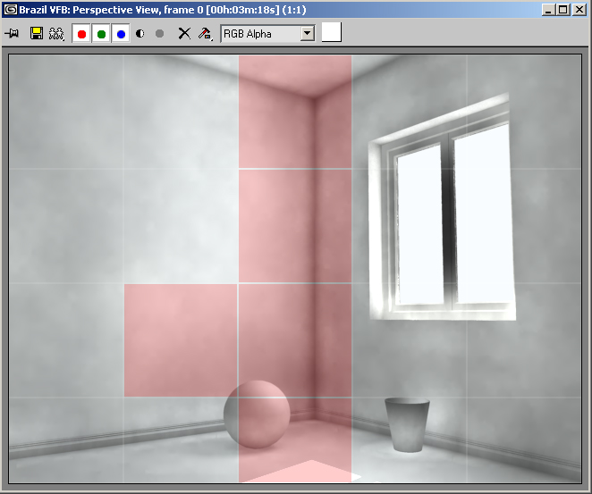
| Pic. 2 Brazil VFB in Select Buckets Mode. Buckets to be rendered are marked with red. The remaining part of the image will be excluded from rendering. This option is very convenient when you configure rendering parameters, because rendering a small part of a scene is much faster than rendering the entire image. You can also configure Brazil VFB so that the previously rendered picture is retained, which makes it convenient to compare the results of modified parameters. Thus, we have a convenient tool to find quickly optimum settings for the final render. However, there are some exceptions. If an image is rendered using only a photon map, you will save minimum time because the photon map will still be built full-scale according to the specified settings. As rendering is carried out in buckets (rectangular cells of a specified size), you can estimate the time it will take to render the entire image by the time spent on rendering several buckets, as the total number of buckets constituting an image is known. And at last the selective render of several buckets can be useful, if you need to re-render only part of an image, for example to change the material on an object. But in this case you should be careful – if you make a lot of changes in rendering parameters, the re-rendered cells may be noticeably different from the other cells, and so a "patch" will appear on the image. The second important advantage of Brazil VFB is its render exposure and color correction controls. They can be used directly by changing parameters of a completed render right in Brazil VFB window. This method is limited in potential, because considerable changes in exposure parameters result in distorted render colors. This tool is also very useful to experiment with exposure settings of a complete render, in order to find out in which direction to proceed. And then the discovered values can be inserted into parameters of the Exposure Control group in Brazil: Exposure/Color clamping. In the latter case exposure values will be used in rendering, but not applied to a completed render, which will provide a final result of a higher quality.
 Pic. 3 Brazil VFB Interactive Exposure Control. Exposure – exposure control is used when an image contains both brightly illuminated areas (hot spots) and dark areas, that is when the dynamic light range does not fit into the dynamic RGB range. Exposure parameter is similar to the exposure notion in photography – the higher its value is, the lighter the image will be and vice versa. Gamma allows to control image contrast, or the difference between light and dark areas. It influences the brightness or fading level of the image. Increased Gamma value results in reduced image contrast. Black Point – using this parameter you can control which RGB color values will be considered black in rendering. Increased Black Point value results in dark areas getting even darker. White Point controls which RGB values will be considered white during rendering. This value reduced will result in brightening light image areas. Combination of Black Point and White Point leads to modified dynamic range borders of a rendered image. For example, by increasing the White Point value you can reduce hot spots in the image. By reducing the Black Point value you can develop image details in dark areas, which on the whole means the enlarged range of colors displayed in a rendered image. Another important setting in this tabbed page – Verbose level in the Console options group. Console is used for feedback from the program core of brazil. It offers sort of a report on results of internal operations of the software brazil engine during rendering. This information may turn out very useful to diagnose various rendering problems and to solve them. Verbose level specifies how detailed this information will be. Minimum level – zero, it provides only general information. Maximum level – the fourth, in this case console can bury you under detailed information on various aspects. You should choose Verbose level reasoning from your conditions. For example, if you have no problems with rendering, you can choose the minimum level or turn off console during rendering. Brazil: Image SamplingParameters in the Brazil: Image Sampling tabbed page are used to control antialiasing (AA). Aliasing involves a wide spectrum of artifacts in rendered images, the main reason of their appearing being discrete values used for analog quantities. The most known effects are jagged object edges, grainy semi-tone transitions (for example, at borders with soft shadows), blinking in animations, etc. There is a mathematical theory developed to eliminate these effects. It lies in refining color values of pixels by disjointing them into constituent parts – subpixels, emitting additional rays through the subpixels and approximating results to the whole pixel. The ground for disjointing a pixel into subpixels is the color difference value between neighboring pixels or subpixels. The process of disjointing pixels into subpixels and emitting additional rays is called supersampling. There also exists undersampling, when one color-determining ray is used for several pixels. Undersampling is used to accelerate calculations when the color of a given area changes rather slowly, so that it can be reproduced accurately enough by interpolating by several control points. Brazil uses adaptive supersampling. It means that you can specify a fork of values for minimum and maximum number of rays per pixel and a threshold contrast value, which will change the number of supersampling rays within the specified range when necessary.
 Pic. 4 Supersampling controls Min Samples – minimum number of rays per pixel or pixel group. Its values are the powers of 2, so 0 means that minimum 1 ray will be used for each pixel to determine color. Negative values will result in undersampling, that is one ray will be used to determine color of a pixel group. In case of values greater than 0 (1 and greater), a pixel will be disjointed into subpixels right away (to be more exact, into a matrix of n x n subpixels, where n is the power of 2 from Min Samples). That is 2 or more rays will be used to determine a color of one pixel. Max Samples – maximum number of rays per pixel or pixel group. It can also take negative, 0, or positive values. Both parameters have the bottom limit of values of 4 (one ray for a 16x16 matrix) and the top limit of 8 – not more than 256x256 subpixels and corresponding rays can be used to determine a color of one pixel. The most widely used Min/Max Samples values: -3 0, -2 -1 or -2 0 for previews; 0 2, 1 2, 1 3 for final renders. Low Contrast – it turns supersampling into adaptive supersampling. Sample color on the right helps you define the contrast value. You can specify the contrast for each RGB channel separately or specify the common value of illumination intensity change by setting the value parameter in the HSV imaging model. Contrast value is used by the brazil engine to decide whether to increase the number of supersampling rays. Here is the algorithm. Firstly, a color is calculated for a pixel or a pixel group according to Min Samples. Then the values of calculated colors of neighboring pixels (pixel groups or subpixels) are compared. If the color difference exceeds the value specified in Low Contrast, the number of rays is increased twofold. It means that the pixel will be split into 2 subpixels, (a group of pixels or subpixels is halved). Color values are again calculated for the new rays and the entire process is repeated. The cycle ends if the difference between neighboring pixels gets less than the contrast value, or if the maximum number of supersampling rays specified in Max Samples is reached. If the contrast is set high, supersampling will most likely involve minimum number of rays. If the contrast is low, supersampling will most likely involve maximum number of rays. You should choose the contrast value for a final render assuming that the human eye can distinguish colors differing 3-4 color grades. New color values determined for subpixels of a single pixel are used to calculate the refined pixel color. Various filters in the Image Filter group on the Brazil Image / Texture Filtering tabbed page are used for this purpose.
 Pic. 5 AA Filters In other words, filters are rules, which are used to determine a pixel color by its subpixels' colors. It should be noted that there is a conclusion in AA theory that a pixel color depends not only on the color of its subpixels but on the color of neighboring pixels as well (ideally – on all neighboring pixels). Many filters used in brazil for AA take this issue into account. The most universal of all available filters is Mitchell-Netravalli. It provides quite a good quality, rapid calculations and detail level. Each filter is shortly described in a text box a little below the list of filters. Jitter Samples – A ray, which is used to determine a pixel (or subpixel) color, usually goes through its center. It very often leads to the appearance of patterns, known as moire. To avoid this undesirable effect, the ray can be allowed a random deviation from center instead of being emitted through the pixel center. Jitter Samples parameter sets random deviations for each AA ray. P1, P2, P3 buttons are preset Min and Max Samples values with constant contrast value=http://www.ixbt.com/soft/25. Thus, the selection of Min and Max Samples, Low Contrast values and a filter determines the method and quality of AA. Brazil Exposure / Color Clamping
 Pic. 6 Exposure / Dynamic Range Controls We have already discussed exposure control above. The other parameters of this tabbed page pertain to color clamping. Brazil uses internal extended precision digital format to render colors. It means that color values are represented by floating point figures and by values beyond the RGB range. On the other hand, imaging in Brazil VFB (like in 3D Max VFB) uses the RGB model. Thus if the image is not rendered in HDRI format, you should control the conversion of internal color representation into the RGB model. Brazil Color Clamping offers several instruments to do it. Clamp Color Range for Render Effects is used together with Render Effects, this option enables the standard mode of clamping the color range used in 3ds max instead of the clamping algorithm used in Brazil. It's recommended when a rendered image contains artifacts. Luminance Compression – compression ratio of color values. True digital color value will be divided by this ratio. Color compression allows to narrow a wide color range, for example to the RGB range with its 255 color intensity grades. This compression helps eliminate hot spots in rendered images to a certain degree. Sampling – this parameter will come in handy if you use an HDR image to light the scene for example. It limits the maximum luminance value per one ray. It allows to exclude separate bright pixels of the HDR image from calculation, which illumination intensity may reach very high values and cannot be eliminated by blurring. Brazil: Ray Server
 Pic. 7 Ray Server Parameters The theory of ray tracing near ideal reflection/refraction angles has been already discussed above. So I hope that the information below will not be difficult to understand. The Ray tracing Depth Control group provides criteria to complete ray tracing. Reflected – ray tracing will be completed after the ray is reflected from surfaces a specified here number of times. Refracted – the same thing but with respect to refractions for transparent surfaces. Total – total number of maximum reflections and refractions. If Total is less than the actual sum of values specified in Reflected and Refracted, random figures come into play – the actual number of reflections and refractions will be random for various surface points, but their total will not exceed the Total value. Auto Cutoff – sets raytracing exit by the value of the returned color. If the color value is less than the Auto Cutoff value, raytracing in this direction is cut off. There are color boxes and texture slots on the right, which help directly specify the color returned by raytracing at the end of the procedure. The Options group allows to calculate various additional effects, such as blurred reflections and refractions (Glossy), self-reflections, etc. Enabled Glossy in Ray Server just allows to calculate this effect, blur settings are actually provided in material parameters. Ray tracing Acceleration is a very important group of parameters. Actually all illumination calculations in brazil, from antialiasing to photon maps, are connected with tracing a certain ray type and calculating their cross points with surfaces. One can literally say that not less than 90% (in fact, may be even more) calculation time is spent on calculating cross point coordinates of the rays. That's why accelerating these calculations has a direct effect on the overall brazil performance. There are a lot of methods to accelerate crossing tests, currently brazil uses so called voxels. The entire scene is subdivided into 3D cells of a specified size (width x height x depth). Each cell contains descriptions of polygons located within its boundaries, and the entire voxel grid is a database with polygon locations. When calculating cross points, real tests are substituted for searching polygons along the ray in the database, and the real crossing tests are carried out for these polygons only. The fewer polygons are within one voxel, the faster ray tracing will be. But increasing voxel quantity requires much RAM, so it's not always possible to reach the limit when one voxel contains one polygon. Voxels can also be subdivided so that their parts contain fewer polygons. Subdivision depth and subdivision criterion can be specified in settings.
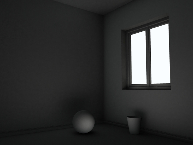
 Pic. 8 Ray tracing Acceleration Settings Mode>Single Grid – the voxel grid. The list also contains another acceleration method – Manual Hybrid, based on creating polygon databases by objects. It's not recommended by developers. Max Size – here you can specify the maximum number of grid voxels. For example, 25 means that the voxel grid cannot be larger than 25 voxels wide, high and deep. The real number of voxels in the grid will depend on the number of polygons in the scene and the Max Polys value. Max Depth – maximum subdivision depth of a voxel, if it still contains more polygons than specified in Max Polys. Be careful with this parameter, because increasing the max depth requires much RAM. Max Polys – polygon counter, criterion to determine the real number of voxels and their subdivision depth. The less the value is (minimum value cannot be less than one polygon), the fewer crossing tests will be done. However small Max Polys values do not always result in overall calculation performance gain, because the program may happen to spend much processing time on building the voxel system. You should always find the optimum ratio between the time for setting up the voxel grid and the time for ray tracing. Balance – this parameter controls the way the voxel grid will be built. With high balance values (about 1), the grid size will be given preference over the voxel subdivision depth when building the grid, that is grids with more voxels will be built, which will not be subdivided (or almost not subdivided). With low Balance values (about 0.5 and lower), the preference during grid building will be given to subdividing voxels. In this case there will be created grids with fewer voxels, but almost each voxel will most likely be subdivided as far as Max Depth allows it. Both methods accelerate calculations, the real effect will depend on a given scene. In Ray tracing Acceleration settings there are three use-proven presets for different situations. You cannot adjust your own settings, you can take advantage of these presets. Low RAM – settings for cases when there is not enough free memory to render a scene. It's not a rare occasion in case of high-polygon scenes. If your scene makes your operating system freeze or results in an abnormal termination of rendering, try these parameters. Though rendering will be real slow. Moderate – average memory capacity, average render time. Max Speed – if there is enough memory to render a scene, use this set of parameters, it will provide high render speeds. This set of parameters may serve as a starting point for your experiments with rendering speed. Brazil: Luma ServerIt's one of the most important tabbed pages in brazil, which contains settings for the two illumination components out of three (raytracing is configured in Brazil: Ray Server reviewed above). We mean direct illumination and secondary diffuse illumination, which can be calculated only by Monte Carlo method. Brazil allows to calculate each of these two illumination components separately. For example, by deselecting the Indirect Illumination>Enable checkbox, we'll force brazil to calculate only direct illumination with raytracing reflections/refractions (they can be disabled as well). This option is very useful at the initial stages of scene setup, when you set up lighting and configure its parameters. |

Pic. 9 Direct Illumination Only. The scene contains three light sources. You can calculate only secondary illumination, starting from the first diffuse bounce and higher. To do that, you should disable Direct Illumination calculation. |
Pic. 10 Illumination from the first diffused bounce only (bounces=1). This option may come in handy to analyze secondary illumination settings.
 Pic. 11 Settings for direct and indirect illumination calculations. Illumination can be enabled or disabled by illumination types (Direct/Indirect) or by light source types. In the Indirect Illumination group you can exclude selected objects from indirect illumination.
 Pic. 12 Adaptive settings of indirect illumination. Brazil does not calculate indirect illumination for every point visible in camera using Monte Carlo method (thereinafter – QMC). The situation resembles supersampling in case of regular AA. At first indirect illumination is calculated for the point groups visible in camera, which quantity equals the power of two, specified in Min. One and the same illumination value found is allocated to all points in the group. Then, illumination values of neighboring groups are compared with each other, and if the difference is greater than the Contrast value, the point groups are split in half and they have their secondary illumination additionally calculated. The process is repeated until the illumination difference of neighboring groups gets less than the Contrast value, or until the number of point groups reaches their maximum quantity specified in Max. Thus, this group of parameters implements the adaptive procedure for calculating indirect illumination. The most often used pairs of Min Max parameters: -4 0 for previews with Contrast from 25 and higher, -3 0 for final renders with Contrast 25 and lower. The Max values greater than zero are rather rare. The higher render resolution is, the lower Min - Max values can be used. All the above-said with respect to adaptive procedure of calculating secondary illumination brings us to the only conclusion – brazil does not use interpolation to calculate secondary illumination at all. In practice it's one of the reasons for slow illumination calculations in brazil as well as for its high accuracy.
 Pic. 13 Settings for indirect illumination calculations using quasi- Monte Carlo method (QMC). The central group of parameters, determining the secondary illumination calculation proper using QMC (quasi- Monte Carlo). As we have already discussed QMC, I will just describe the settings. Sampler – a list of calculation algorithms, which presently contains only one element - Quasi Monte Carlo. View Rate – the number of sampling rays in a semisphere (rays emitted through the semisphere surface built around the point visible through camera) to calculate secondary illumination. These rays are traced in the scene up to the first crossing with the nearest surface. The new points, obtained from these crossings, have their direct illumination calculated. This is the first bounce or the first diffuse reflection, as the light falls to the surface, is diffusely reflected from it and gets to the point visible from the camera. Besides the direct illumination, ray tracing is done for these new points, results of calculated illumination are also returned to the starting point. And finally, indirect illumination has to be calculated for the new points. So these points have their own semispheres built around, sampling rays again being emitted through them. The number of such rays is specified in the Sec Rate parameter, and the number of times the entire process is repeated is specified in the Bounces parameter. When a sphere around a visible point is being sampled, the first light bounce or the first diffuse reflection is calculated. The first bounce gives a new set of points, sampling its spheres provides the second bounce calculation, which in its turn results in the appearance of a new set of points, sampling these points gives the value of the third bounce (diffuse reflection) etc. That's why the Bounces parameter is also called a tracing depth of indirect illumination. The higher the tracing depth is, the more accurate diffuse illumination calculation will be and the longer it will take to be calculated. The higher View Rate and Sec Rate are, the less is the noise, the smoother is a rendered image, and the longer is rendering. The View Rate value within 5 – 15 can be used for previews. Use 40 and higher for final rendering. The Sec Rate value, recommended by developers, must be a half or three thirds of the View Rate value. Parameters of the Indirect Energy filter group are multipliers of calculated intensity and color of the calculated illumination. They can be used to reduce intensity of the secondary illumination (Diffuse or Specular lower than 1) or on the contrary, to increase it. Color boxes in this group allow to specify the color of secondary illumination. Thus, QMC allows accurate calculations of all three illumination components. But it will take up much time to calculate. Besides, QMC cannot calculate caustic-effects of the illumination alone. Among the shortcomings of the QMC method of calculating illumination in brazil one can name the impossibility to save illumination calculation results into a file, necessity to recalculate illumination completely after you change AA settings or exposure control, lack of interpolation or any settings of the QMC properties. You can use QMC alone to calculate secondary illumination, or use it in combination with the method of photon maps. This calculation method is called regathering. In this case QMC calculates only the first bounce, evaluation of the illumination from the second and further diffuse multiple reflections is taken from the photon map. This method provides high quality and faster calculation in comparison with the "pure" QMC. In case of regathering, the Bounces parameter also performs an additional function. If a photon map is activated for calculations and Bounces=1, the secondary illumination is calculated only by the data from the photon map, QMC is not used at all. If a photon map is activated and Bounces=2 and higher, the first bounce is calculated by QMC, the rest – the photon map. If a photon map is not activated, all the calculations are carried out by QMC, and the Bounces value determines the depth of bounce tracing. Brazil: Photon Map ServerPhoton Map Server is the heart of photon map configuration.
 Pic. 14 Photon map type selection There are two types of photon maps – Global, used to create photon maps for calculating indirect illumination of the entire scene, and Caustic, used to calculate caustic effects of illumination for separate scene objects. This division is determined by the fact that caustic effects require high photon density, which is difficult to provide using a global photon map. High photon density is achieved due to locality, that is a caustic photon map is created for a small surface area, so that you can reach high caustic photon density even with a relatively small quantity of caustic photons emitted by a light source. You should specify a source object and a recipient object to calculate caustic effects. Any object, which surface possesses mirror reflection or transparency properties, can be used as a source. As a recipient, you'd better use objects with surfaces possessing only diffuse properties. For example, caustic effects can be calculated for a glass on a table. In this case the glass walls will act as the caustic source, and the table surface will be the recipient. If the surface of a source object is curved like a lens, caustic effect will be more prominent. The nature of caustic effects is connected with the refractions in transparent and reflecting surfaces, which focus diffuse light into a thin beam after refraction or reflection. If the map type is active, it's indicated by a green light next to the map type. Photon map statistics are also provided here – its prospective size, the number of actually stored photons, allocated memory capacity, and the cache status of a photon map. The data change in the process of photon map generation.
 Pic. 15 Photon tracer settings. Here you can control the strategy of creating a photon map and the tracing depth – total number of photon reflections from surfaces. Prepass Type – this parameter selects a strategy for creating a photon map. Actually, it's rather difficult to forecast the total number of photons stored in a photon map, though the number of photons emitted by the light source is always known. The reason is that when photons are reflected from surfaces, the randomness factor (aka Russian roulette) comes into play. Using a random number generator taking into account such surface properties as diffuse or mirror reflection/refraction of a material, Russian roulette determines what will happen to a photon – whether it will be diffused or reflected at a mirror angle, or will be absorbed. Indeterminate character of a photon map capacity is only amplified with the number of photon bounces increased. That's why the brazil photon server makes a prepass, emitting a small part of photons. Judging from the stored results for this small part, the program estimates the total number of photons that will be stored after all of them are emitted. This will be done, if Prepass Type is set to Map Size. The estimated figure is displayed in Map Capacity of the corresponding map type. If the #Emitted type is selected, the photon server emits photons so that the number of photons stored in a map corresponds to the total number of photons, specified in emission parameters of light sources. It's convenient when you have to get a strictly specified number of photons stored in a map. Splitting – this option forces the photon server to differentiate between the photons reflected from surfaces and the photons passed through a transparent surface. It helps reduce noise in caustic effects. This option is useful when used together with a caustic photon map, it is not necessary to calculate a global photon map. In the latter case, you had better disable this option, as additional memory is required to differentiate between the photons. Diffuse Depth – maximum number of diffuse multiple reflections, which a photon can undergo. This number of reflections reached, the photon is not traced. You should take into account that each collision is recorded in a photon map. So if you specify a great number of reflections, the resulting size of a photon map can be quite imposing even with a small number of photons emitted from light sources. Reflected Depth / Refracted Depth – the same thing regarding mirror reflections/refractions of photons. A photon record will not be stored until it reaches a diffuse surface.
 Pic. 16 Irradiance Estimate settings. This group allows to a certain degree to control estimation of the irradiance of a point visible from camera. Photon map is a database that stores coordinates of photon collisions with surfaces, photon energies, and their direction of incidence on the surface. So, when you need to calculate illumination of a surface point, the database is searched by the point coordinates for photons, which are either within the circle of the specified radius (Max Search Radius) with the center in this point, or within the specified number of nearest photons (Photons in Estimate). Energies of selected photons are added together with some weight ratios producing a point irradiance estimate. We are speaking of an estimate, not an accurate irradiance value, because estimate accuracy heavily depends on the photon map density. The higher the density is, the more accurate the irradiance estimate is. Another important note concerns the interaction of Photons in Estimate and Max Search Radius parameters during the estimation process. These two parameters are competing – if one of them is reached earlier, the other will not be used. For example, if Max Search Radius is reached earlier than Photons in Estimate when estimating the irradiance, the photon search stops, though the actually collected number of photons does not correspond to the specified value. And vice versa. It should be taken into consideration, because the Photons in Estimate value has a direct impact on render smoothness, and Max Search Radius – on the secondary illumination accuracy. Considering the importance of these two parameters, let's analyze their interaction peculiarities. One of the fundamental properties of a photon map is the quantitative relationship between the number of photons collected for irradiance estimation, photon map density in the irradiance estimate point, and the photon search radius. This quantitative relationship can be expressed in a simple formula: (Actual number of collected photons) = (local density of the photon map in the irradiance estimate point) x (actual area of photon search within a circle of a given radius) I mean actual values, because manually specified data for the corresponding parameters will not always coincide with the values, which will actually be used to search photons. For example, you can specify 5 meters as a photon search radius, set the number of collected photons to 10, while the actual photon search radius will be much less than 5 meters even for a photon map with low density, because the condition of 10 collected photons will be reached much earlier. Another example. If you set the number of collected photons to 10 000 and the photon search radius to 1 mm, the real number of collected photons will hardly exceed 1000 even for a photon map of a high density, because the maximum search radius will be achieved much earlier. So, the main property of a photon map can be used to determine one of the parameters using the other two, if their values are known. Approximated actual value of Max Search Radius (a radius of photon collection to estimate irradiance) can be determined, if you know the average density of a photon map and if you specify Photons in Estimate. Approximated actual value of Photons in Estimate (a number of collected photons to estimate irradiance) can be determined, if you know the average density of a photon map and if you specify Max Search Radius. We are talking about approximated values, because a photon map density, including the search radius and the number of photons collected, will be different for different surface points. It's important to be able to determine Photons in Estimate and Max Search Radius, because render smoothness and secondary illumination calculation accuracy depends on them. Thus, the above mentioned formula sets the direction where to search for settings depending on what render you need to obtain – just a smooth picture, or a smooth picture with accurate secondary illumination at a certain density of a photon map. And even if you don't use this formula to determine quantitative values of these parameters, understanding its qualitative content is very important to work successfully with photon maps. It's rather difficult to devise a formula to calculate a photon map density by the number of emitted photons, and it's not necessary either. That's because the approximated density of a photon map is easy to determine in practice. I'll write how you can do it later. Density of a photon map can be considered a unique property of a certain scene, because it directly depends on the scene geometry, properties of the surface materials and light sources. Of course, density of a photon map will also depend on the number of emitted photons, but the density of a photon map will be different for different scenes with the same number of emitted photons. One can even assume that the ratio of emitted photons and the density of the photon map will be a constant value, which will label a scene like a finger-print. But the analysis of this property is not the object of this article, so let's skip it. Let's return to irradiance estimate parameters. Estimator – algorithm of estimating irradiance. There are three options – Basic, Advanced, and Analysis. Basic is the simplest and the fastest algorithm out of the three, but it does not support many important functions. For example, it treats wrong thin surfaces and it cannot create mirror highlights, it calculates wrong bump map shadows. So the speed is its only advantage. It's rarely used. Advanced – full featured irradiance estimate algorithm, it can do everything that Basic cannot, but it works more slowly. This is the default algorithm in brazil. Analysis is a special algorithm for finetuning irradiance estimate settings, especially the photon search radius and the photons in estimate. Rendered using this algorithm, the program returns colors which can be used for the analysis. At present only the red color provides useful information. If there is no red color in a given area, it means that there are enough photons in this area to estimate irradiance or that there are less than 8 photons. The brighter the red color is, the bigger the error is and the higher the shortage of photons is to estimate irradiance. |

Pic. 17 Image rendered in the Analysis mode. Red spots indicate insufficient number of photons to estimate irradiance – these are areas where it's impossible to collect the number of photons specified in Photons in Estimate, within the radius specified in Max Search Radius. Search type – photon search type for an estimate near corners and joints. There are two types: Spherical and Elliptical. Elliptical is more accurate with corners, but it's slower than Spherical. Specular – this option enables calculating mirror highlights using a photon map. This function supports only materials of the Brazil BasicMtl type so far.
 Pic. 18 The other photon server settings. Photon Energy>Multiplier allows additional control over the photon energies to configure illumination brightness in the scene. Besides, there is another photon energy control in light source settings. Developers do not recommend setting this multiplier higher than 1, because it may lead to artifacts. As an alternative you had better control photon energies in light sources. Filtering – conic filter, which is used in estimates. It determines weight coefficients for added photon energies, so that remote photons contribute less. For a global photon map this filter provides additional smoothing of the calculated illumination, in case the filter size is correct and regathering is not used. For a caustic photon map this filter allows sharper effects, increased filter size results in blurred caustic. Cashing – stores a photon map in RAM, which allows not to recalculate it for each render. Caching is useful when a photon map is not large in size and when rendering animations. Photon Map Files – allows to store the calculated photon map into a file. This option is a must when setting up a photon map, because changes in Max Search Radius and Photons in Estimate do not require recalculating the photon map. That's why they can be changed while loading the same photon map from file, which is much faster than recalculating it. File – here you specify a folder and file name to store a photon map. |

Pic. 19 Direct illumination and indirect diffuse illumination, calculated using a photon map. |

Pic. 20 Photon map only, photon tracing depth – 20 diffuse bounces. |

Pic. 21 Regathering, the first diffuse bounce is calculated using QMC, the rest – using a photon map. We have reviewed photon map parameters in much detail because of the very important role played by Global Photon Map in obtaining high quality illumination calculations during rendering. Summing it all up, I can tell that most efforts to set up rendering with a photon map are actually spent on choosing a photon map size (the number of stored photons) and on looking for appropriate values for Max Search Radius and Photons in Estimate. We also need to review some source light settings, which concern photons. Light SourcesThey are undoubtedly the most important factor for setting up illumination. But we shall review in detail only those parameters, which concern indirect illumination. Brazil offers light sources for all main source types in 3ds max plus two area light sources. Thus, we have 5 light sources: omni, spot, directional, rectangle area, and disk area. The main advantage of light sources in brazil is their capacity to emit photons. In light source settings you can separately enable/disable different illumination types – direct and indirect. Thus, you can enable illumination type calculations in three places in brazil – from the light source control panel (in two places) and from the render control panel. This is certainly a very flexible approach. Nevertheless, if you forget to enable a light type at least in one place, it will not be calculated. Taking into account that the control panels are scattered in various places of the interface, it's not very convenient to control. All light sources can be photometric and they can use real physical illumination parameters, such as 3D illumination distribution and illumination intensity units. Indisputable advantage of brazil is its built-in IES file viewer. If photometric lights are not used, illumination brightness is set on the Color/Projector tabbed page. Here you can set the illumination intensity and its color. When calculating illumination from light sources, their emission type is taken into account. We should dwell on area lights, as they possess the diffuse emission type – illumination from each area light will depend not only on the distance, but also on the angle between the direction to the area light and the normal of the point, where the illumination is calculated. Illumination from area lights is based on subdividing their surfaces into a grid of areas. Each area is sampled by one or several rays. Illumination in a point is a total of sample illuminations for the light source areas visible from that point. There are two main algorithms in brazil to calculate samples – Regular and Adaptive Halton, which are available on the Area Light Options tabbed page.
 Pic. 22 Area Light Options. Regular uses a constant number of samples, Adaptive Halton changes the sample number depending on illumination conditions. For example, when part of the light source is blocked by an object, more samples can be used in the border area. Initial start – specifies the initial number of samples. It remains constant for Regular and can be changed for adaptive sampling. The 1 and higher values are recommended for regular, for adaptive sampling – small initial start values within 0.1 or lower. Error estimator – the way to estimate an error in calculating illumination. There are three types – mono, RGB, and HDRI. Mono is faster, but it can result in noises in colored shadows or when illuminated by a colored texture. RGB guarantees that the error will not exceed a specified value in all color channels. HDRI is more accurate in estimating the error in shadows and it's the slowest of the three error estimators. Max samples – maximum possible number of samples, this number cannot be exceeded no matter how the adaptive sampling is configured. Estimate intrvl – interval for calculating the sampling error. The larger the interval is, the more accurate and the slower the error will be calculated. Max error – the main setting that enables additional sampling and determines the quality of illumination calculation. It is a ratio percentage of the error value to the global illumination value. For a final render you'd better use the Max Error of 0.1% and lower in combination with high max samples, about 1000 or even higher. Max error can be high for a preview, up to 100%. As area lights may considerably slow down calculations, spot lights can be used as their alternative, as they can also emit photons and brazil allows to calculate shadows for these lights as well, like for area lights. Calculating indirect illumination is based on real physical laws, that's why the choice of attenuation type together with the choice of real units and real geometry sizes is crucial. Attenuation type can be selected on the Attenuation / Decay tabbed page.
 Pic. 23 Attenuation Type Selection. Decay>Auto is used for photometric light sources, ON allows to select the quadratic Inverse Square attenuation from the drop-down list (you should use this attenuation) or distance-proportional attenuation, OFF completely disables attenuation. The Attenuation group also allows to specify clipping planes of the illuminated scene area. In this case the illumination will be only between the selected planes, which is convenient to cut down the calculation time. In case of the Inverse Square attenuation you should also specify the initial point relative to the light source, from which the attenuation will start, and Scale, which allows additional scaling of selected units. If real units are selected, Scale can be set to 1 and the illumination can be controlled by its intensity and energy (for photons) settings. Or you can leave intensities and energies alone, and increase the Scale value instead. The latter method is more convenient, and besides, changes in illumination intensity are displayed in the Max workplace. And finally, the Photon Maps tabbed page.
 Pic. 24 Settings of properties and quantities of photons emitted by a light source. That's the place where you should specify the type of emitted photons, Caustic or Global, the number of photons emitted, and their energy. This tabbed page also houses additional photon emission parameters. But as developers are not sure whether these settings will be retained in the next brazil version, we shall not review them and will limit ourselves to default photon emission settings. Schemes and Strategies for Calculating IlluminationThe main purpose of this review is above all to analyze brazil configuration methods and means for indirect illumination calculations. And many other issues, important for illumination on the whole, are left out of the scope of this article. For example, setting up direct illumination and materials. However, this approach is justified, because it allows better focus on the object of the article. Later on, both direct illumination and materials, as well as other topics, will surely be touched upon in descriptions of sample illumination settings for certain scenes, but only as much as necessary. Indirect illumination calculation setup pursues only two objects in the long run. The first one – to obtain smooth rendered images with secondary illumination, without visible patches, hot spots/dark areas in the corners and other artifacts. The second – to obtain physically correct secondary illumination while preserving smooth rendered images. The latter task is much more difficult, it requires more time and efforts. There can be three methods of calculating secondary illumination.
All the three methods of calculating illumination in brazil are used in practice and their examples will be reviewed in much detail in the next, second part of the review. See you!
[an error occurred while processing this directive] |